Effective Data: Partition
Published
To train a good model, you need lots of data. Luckily, over the last few decades, collecting data has become much easier. However, data is still a major constraint for most large-scale Machine Learning projects along with computational power.
There is an art to collecting data. One popular technique used especially in image recognition and detection is Data Augmentation. A single picture can be flipped, rotated, cropped, or recolored to create “new” data.
However, there is little value to data if you use it incorrectly. Even if you double or triple the dataset manually or through data augmentation, without proper partition of data, you will be left clueless on how helpful adding more data was. In fact, if you partitioned your data correctly, you might have concluded that you didn’t need more data!
Train
The most naïve way of using data is to allocate all data to the training set, the set used for training the model. This is definitely not recommended for any real projects, but it may work for simple examples just to test theoretical concepts. Because there is no data allocated to test the trained model, the problem must be simple enough so that a human could easily look at the model to evaluate its accuracy.
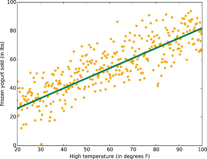
Above is one case where it is somewhat acceptable to allocate all data to the test set. You assume that there is a linear correlation between temperature and sales of frozen yogurt and want to predict frozen yogurt sale. In this simple model, you can visualize the data and the model with a 2D plot, so it is easy to evaluate the model.
However, in most models both the data and the model is obscure, and it is impossible to evaluate the model by looking at plots. Therefore, in any project, some data is allocated for the test set.
Train - Test
The Train - Test partition is a significant improvement to the first “partition.” You allocate most of the data to the training set but leave enough data for the test set. The test set allows you to objectively evaluate the performance of your model.
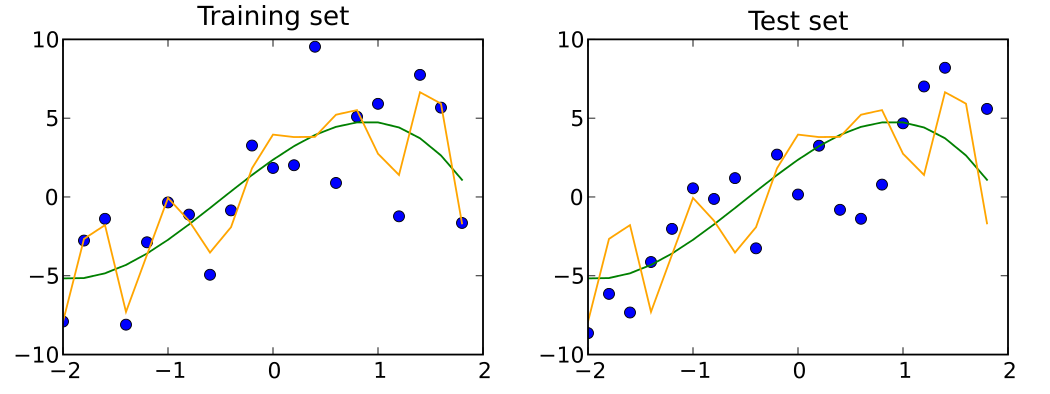
Take a look at the orange model above. For the training set (marked by blue points on the left diagram), the model performs quite well. However, for the test set (the right diagram), the model performs poorly. The model has overfit the training set.
By partitioning data for the test set, you can now detect overfitting models. You should fix them! There are many regularization techniques to address overfitting, but all of them require hyperparameter tuning. You could tune your hyperparameters with the test set, but that is an ill-advised idea. Generally, you should allocate some data just for hyperparameter tuning.
Note that if you do train your hyperparameters with the test set, the test set no longer functions as a test set and should be called a dev set.
Train - Dev - Test
If you tune hyperparameters with the test set, you have the risk of overfitting the test set. With just the training set and the test set, it is impossible to detect whether or not the model has overfit the test set. Therefore, instead of using the test set to tune hyperparameters, you allocate some data to the development set (also called the cross-validation set). Now, the test set is no longer used to tune the model, and it can again be used as an objective evaluation metric for the model. Also, in the rare case that you overfit the dev set, you can detect and fix it.
| Partition | Error |
|---|---|
| Training Set | 0.5% |
| Development Set | 4.6% |
| Test Set | 5% |
Suppose that you have a large difference in error between the training set and the test set like the table above. In this case, the difference between the training set and the development set is large. Since the only difference between the two sets are their data points, you can conclude that the model has overfit the training set.
| Partition | Error |
|---|---|
| Training Set | 0.5% |
| Development Set | 0.6% |
| Test Set | 5% |
Now suppose that you find that the error for training and the development set is similar, but the you get a error spike for the test set. Then you can then conclude that the model has overfit the dev set, and that you should enlarge the dev set.
This partition should be your default partition. This partition is very effective because each dataset is only used for one task. The training set is used to tune the parameters of the model. The dev set is used to tune the hyperparameters of the model. The test set is used to evaluate the model. Because of this clear division, you can easily deduce the primary factor of the error.
Train - TrainDev - Dev - Test
Although the standard Train - Dev - Test partition works well in most times, sometimes you need another partition. Consider you want to build a self-driving car model using the black box camera. Unfortunately, you have a small amount of data. So, you decide to use a game to simulate the traffic and get data. Now you might have enough data to train the model, but the data is a mix of simulated and real data.

Then, how would you divide this mixed data? Because your goal is to train a model that drives a car in real life, your dev set and test set must have data from real life. Then, the only place the simulated data belongs to is the training set. Therefore, your training set and dev set has different data sources.
Then, using the Train - Dev - Test partition can be problematic. Suppose you have 1% error from the training set and 5% error from the dev set. Before, we could infer that the model is overfitting because the only aspect that changed from the training set and the dev set was the data points. Now, not only are the data points different, but also the data source has changed. Maybe the 4% difference comes from the data mismatch between the training and the dev set, or maybe it comes from overfitting. We can no longer infer the cause of error.
Therefore, we need to add a new partition called the Train-Development set. The data from this set is also simulated. Then, when comparing the train set and the train-dev set, only the data points changed.
| Partition | Error |
|---|---|
| Training Set | 1% |
| Training-Development Set | 4.8% |
| Dev Set | 5% |
Now, we can solve the problem we encountered. Suppose that we get a 4.8% error from the train-dev set. Then, the error spike is between the train set and the train-dev set, so we can conclude that the model is overfitting.
| Partition | Error |
|---|---|
| Training Set | 1% |
| Training-Development Set | 1.1% |
| Dev Set | 5% |
Now suppose that we got an error of 1.1% from the train-dev set. Then, the train set and the train-dev set has similar error, so the model is not overfitting. However, there is an error spike between train-dev set and the dev set, so the error can be attributed to the data mismatch.
Therefore, by adding the train-dev set, you can once again infer the primary cause of error.
Conclusion
You have now learned 4 different partitioning schemes for data. The default choice for partitioning data is the Train - Dev - Test partition scheme. If you end up using simulated data, Train - TrainDev - Dev - Test partition scheme should be your default. For simpler projects where you don’t need objective evaluation, you could consider using the Train - Dev partition scheme.
You now know what partition scheme to use! The natural next question would be how large each partition is. One naïve way would be to divide data equally, but there are more effective partition sizes. In my next post, I will discuss the optimal partition sizes.
This post was inspired by Structuring Machine Learning Projects, the 3rd course of Andrew Ng’s Deep Learning Specialization.