Title: Neural Fitted Q Iteration - First Experiences with a Data Efficient Neural Reinforcement Learning Method
Author: Martin Riedmiller
Affiliation: Professor at University of Onsabruck
Current Affiliation: Research Scientist at DeepMind

Prerequisites

• Reinforcement Learning: An Introduction 2nd Edition Part 1 (Sutton and Barto, 2018) [PDF]

Accompanying Resources

• Generalization in reinforcement learning: Safely approximating the value function (Boyan and Moore, 1995)
• Self-improving reactive agents based on reinforcement learning, planning and teaching (Lin, 1992)
• Tree-Based Batch Mode Reinforcement Learning (Ernst et al., 2005)
• A Direct Adaptive Method for Faster Backpropagation Learning: The RPROP Algorithm (Riedmiller and Braun, 1993)
• Least-Squares Policy Iteration (Lagoudakis and Parr, 2003)

Download

• Original PDF
• Annotated PDF

1 Introduction

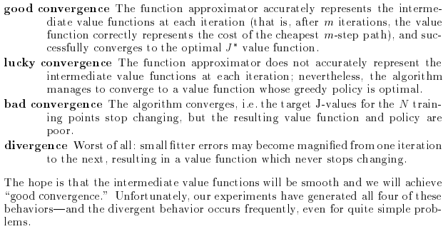
To handle real-world problems with massive scale, reinforcement learning must be accompanied with powerful function approximation methods. However, function approximation is a double-edged sword: its generalization effects can accelerate learning, but weight changes could also negatively affect learning in regions less frequently visited. Boyan and Moore (1995) showed that function approximators lead to poor convergence properties even in simple problems.

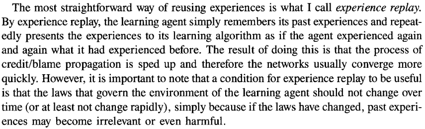
To prevent the agent from forgetting meaningful knowledge, we propose reusing previous knowledge. We store all previous experiences in the form of state-action transitions. Then, for every update, the entire batch of stored experience is reused to update the neural network. This can be seen as a special form of experience replay proposed by Lin (1992).

This algorithm belongs to a family of fitted value iteration algorithms, a family of value iteration algorithms paired with function approximation. Various function approximations are possible, including randomized trees by Ernst et al. (2005).

This algorithm differs by using a multilayered perceptron (MLP), and is therefore called Neural Fitted Q Iteration (NFQ). The paper focuses on the following three properties of NFQ:

1. NFQ is model-free.
2. NFQ is data-efficient due to experience replay.
3. NFQ shows comparable results to analytically designed controllers.

2 Main Idea

2.1 Markovian Decision Processes (MDP)

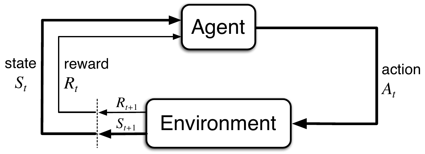
We expect the readers to be familiar with Markov Decision Processes (MDPs). An MDP can be described by a set of states $S$, set of actions $A$, a stochastic transition function $p(s, a, s’)$, and a reward function $r: S \times A \to \mathbb{R}$. Unlike most current reinforcement learning papers that use the reward function $r$, this paper uses the cost function $c$. Thus, the objective of the agent is to find an optimal policy $\pi^* : S \to A$ that minimizes the expected cumulative cost for each state.

2.2 Classical Q-Learning

We also expect the readers to have basic knowledge of classical tabular Q-Learning algorithm. Again, note that we use the minimum of all actions since we use the cost function $c$.

\[Q_{k+1} (s, a) := (1 - \alpha) Q(s, a) + \alpha \left( c(s, a) + \gamma \min_b Q_k (s', b) \right)\]

where $s$ is the state before the transition, $a$ is the action applied, $s’$ is the state after the action, $\alpha$ is the learning rate, and $\gamma$ is the discount factor. Q-learning is guaranteed to converge to the optimal action value $q^*$ for finite $S$ and $A$ if every state-action pair $(s, a) \in S \times A$ is updated infinitely often.

Typically, Q-Learning updates are done online in a sample-by-sample manner.

2.3 Q-Learning for Neural Networks

Vanilla value iteration can only be used in finite number of states and actions. By using function approximation, we can ease the restriction on the number of states and allow $S$ to be continuous. To integrate neural networks into Q-learning, one small change must be made. Because Q-values are no longer stored in a tabular manner but instead encoded in the neural network, we need to compose an error function to update the weights of the neural network through backpropagation. One such error function would be the squared error of the current Q-value and the target Q-value.

\[error = \left( Q(s, a) - \left( c(s, a) + \gamma \min_b Q(s', b) \right) \right)^2\]

We could naively use the same sample-by-sample online updates. However, such approach has shown to result in slow and data-inefficient learning. Weights adjusted from one state-action pair has unpredictable effects on other pairs throughout the state-action space. Although in many cases this allows for generalization and accelerates learning, it is also the main reason for unreliable and slow learning.

3 Neural Fitted Q Iteration (NFQ)

3.1 Basic Idea

NFQ replaces online single-sample updates with offline batch updates. Using batch updates allows for advanced supervised learning methods that are faster and more robust to hyperparameters. Of many advanced supervised learning methods, We use Rprop by Riedmiller and Braun (1993), which frees us from tuning hyperparamters related to the neural network. This allows us to focus on tuning the hyperparamters directly related to reinforcement learning instead of diverting our attention to hyperparamters related to the supervised learning part.

The sample set $D$ is collected by interacting with a real or simulated environment. Each experience in the sample set $D$ is a 3-tuple $(s, a, s’)$, where $s$ is the original state, $a$ is the chosen action, and $s’$ is the resulting state. It is also commonplace to include the reward / cost received to the tuple. However, we perceive the immediate cost as something specified by the designer instead of something observed by the environment. Thus, we leave out costs and specify it at a later point.

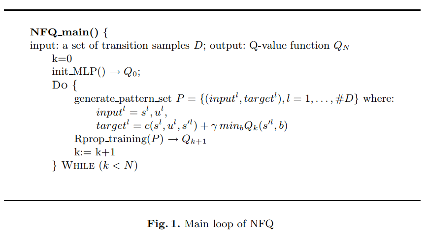
3.2 The NFQ - Algorithm

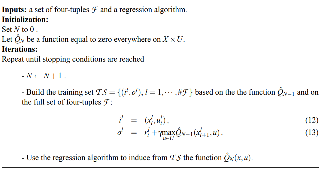
The NFQ algorithm consists of two steps:

1. Generate the training set (pattern set) $P$ from the sample set $D$. $P$ consists of pairs of input $(s, a)$ and target Q-value $c(s, a, s’) + \gamma \min_b Q(s’, b)$, generated from transitions $(s, a, s’) \in D$.
2. Train the neural network with the training set $P$. The training is repeated for several epochs.

3.3 Sample Setting of Costs

As we have mentioned previously, we do not save the cost in the transition samples $D$. This is because we view the cost as a product of design, not something given by the environment. Although NFQ is not bound to any particular type of cost function, we found it useful to standardize the cost function to setup the learning problem. Thus, we design the cost function by partitioning the set of all states $S$ into three sets:

• Goal states $S^+$: The region where the system should be controlled to and kept in.
• Forbidden states $S^-$: The region that must be avoided.
• Other states: States that are neither the goal states nor the forbidden states.

We define the target differently for each set of states:

$$ target = \begin{cases} c(s, a, s') & \text{if } s \in S^+ \\ C^- & \text{if } s \in S^- \\ c(s, a, s') + \gamma \min Q(s', b) & \text{else (standard case)} \end{cases} $$

If the state ends in goal states $S+$ or forbidden states $S^-$, the episode is terminated. Thus, the target is simply the immediate cost $c(s, a, s’)$ or $C^-$. In other states, the costs from the remainder of the episode must also be considered, so $\gamma \min_b Q(s’, b)$ must be added.

For simplicity, we use a simplified version where the cost function is constant for all non-forbidden states. This makes the problem a minimum-time controller problem, where the task is to reach the goal states as soon as possible. This is often desirable in technical process control. We also set $C^-$ to $1$, since it is the maximum possible output of the neural network (due to the sigmoid activation function in the output layer).

$$ target = \begin{cases} c_{trans} & \text{if } s \in S^+ \\ 1 & \text{if } s \in S^- \\ c_{trans} + \gamma \min Q(s', b) & \text{else (standard case)} \end{cases} $$

We can modify the target slightly to make it valid for environments where the task is to stay in the goal region as long as possible, instead of simply reaching the goal. These problems are called regulator problems. In this case, the immediate cost is 0 at the goal states, so the target is just the estimated cumulative cost afterwards.

$$ target = \begin{cases} \gamma \min Q(s', b) & \text{if } s \in S^+ \\ 1 & \text{if } s \in S^- \\ c_{trans} + \gamma \min Q(s', b) & \text{else (standard case)} \end{cases} $$

3.4 Variants

We discuss two possible variants of the basic NFQ algorithm. The first variant is about how the sample set $D$ is collected. In the basic algorithm, experiences collected in $D$ are “random rollouts”: the experiences are from interactions with environment through random play. However, this might result in an incomplete set of experiences to find the optimal policy. Thus, instead of random rollouts, we consider a variant where training samples are collected by greedily exploiting the current $Q_k$ function.

Another variant is to add an “artificial” training pattern called the hint-to-goal heuristic. This artificial data is useful since by definition their target value is 0, so training on these synthetic data “clamps” the value function to 0 at the goal region $S^+$. Since the goal region is defined as part of the problem, it is possible to synthetically generate training data in the goal region.

4 Benchmarking

4.1 Type of Tasks

To test the NFQ algorithm, we define three basic control problem:

1. Pole Balancing (a.k.a. Inverted Pendulum): Avoid forbidden states $S^-$
2. Mountain Car: Reach goal states $S^+$
3. CartPole: Reach and stay in the goal states $S^+$

4.2 Evaluating Learning Performance

There are two important evaluations for learning agents: the speed of learning and the performance. Let’s first discuss the speed of learning, or the “learning performance.” This can be measured with various valid statistics:

• Number of episodes
• Number of cycles (steps)
• Number of updates
• Absolute computation time

Among these, we select the number of cycles (steps) needed to achieve certain performance as the primary measure, complemented with number of episodes. The ‘number of cycles’ measure is useful since it is directly correlated to the number of interactions with the environment. In many real systems, interactions with the environment is the most likely bottleneck factor, so this measure can accurately evaluate the learning performance of the agent in real systems.

4.3 Evaluating Controller Performance

Now, let’s discuss how to evaluate the performance of the agent. It is commonplace to define an episodic “cost measure” and average them over some number of episodes. For minimum-time controller problems, we use the average time to goal as the cost measure. For regulator problems, we measure the total time outside the target region.

Note that the learning controller can have a different internal goal formulation different from performance measure, either through reward shaping or discounting. In other words, the learning controller could seek to minimize a cost measure different from the cost measure used for evaluation.

To evaluate the controller accurately, we must specify the “working region”: the set of starting states for which the controller should work. This working region could be a single starting state, a finite set of starting states, or a region within the set of all states $S$. We use the third case, which is the most general and typically the most challenging case.

5 Empirical Results

All experiments were performed using $CLS^2$.

5.1 The Pole Balancing Task

In Pole Balancing, the agent’s task is to balance a pole at an upright position by applying left, right, or zero force every 0.1 second. The states are represented by the pole angle $\theta$ and the angular velocity $\theta’$. The states are partitioned as follows:

State	Condition	Cost
$S^+$	$\theta \in [-\pi/2, \pi/2]$	0
$S^-$	$\theta \not\in [-\pi/2, \pi/2]$	1

Three actions are available to the agent:

1. Apply left force ($-50 N$)
2. Apply right force ($50 N$)
3. Apply zero force ($0 N$)

A uniform noise of $[-10, 10]$ is added to the chosen action.

(For more details about the environment, please read Section 9.2 of Least-Squares Policy Iteration by Lagoudakis and Parr (2003))

Learning System Setup

The sample set $D$ was generated by starting the pole in an upright position and then applying random actions until failure.

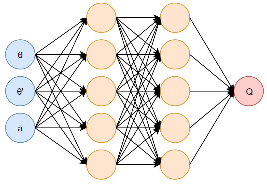
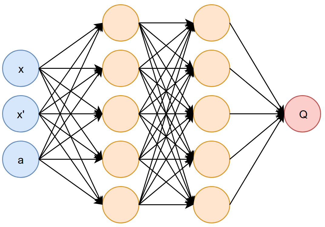
To approximate the Q-value, we use a multilayer-perceptron with two hidden layers. The input layer has 3 nodes: 2 for the state $\theta, \theta’$ and 1 for the action. The hidden layers have 5 nodes each, and the output layer has 1 node. A sigmoid activation was used in all output. We used the discount factor of $\gamma = 0.95$.

Results

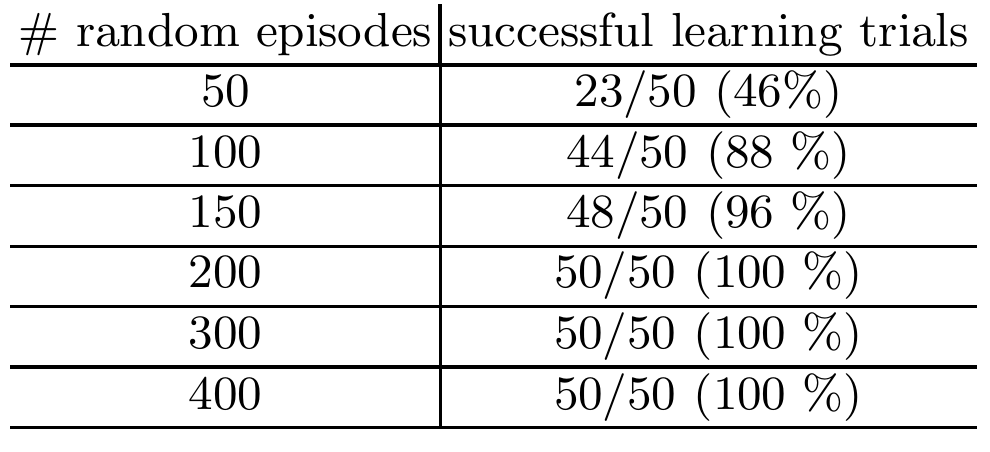
To evaluate the speed of learning, we vary the number of training episodes from 50 to 400 episodes. After training, the controllers were tested on 50 test episodes. Controllers that trained with 200 or more episodes (roughly 1200 steps) were able to pass all 50 test episodes.

5.2 The Mountain Car Benchmark

In Mountain Car, the agent’s task is to accelerate the car up to the top of the hill. Unfortunately, the agent’s car is too weak to drive directly up the hill, so the agent must learn to move in the opposite direction to gain momentum. In this task, a state is represented by the position $x$ and the velocity $x’$.

State	Condition	Cost
$S^+$	$x \geq 0.7$	0
$S$	$x \in (-1, 0.7)$	0.01
$S^-$	$x \leq -1$	1

Two actions are available to the agent: left (-4) and right (+4).

Learning System Setup

To generate the sample set $D$, initial starting states were drawn randomly such that $x \in (-1, 0.7)$ and $x’ = 0$. Instad of using random actions, the actions for the training episode were generated by the controller, greedily exploiting the current Q-value function. Each training episode had a maximum length of 50 steps. We also use the hint-to-goal heuristic, where we generate artificial data in the goal region. After every training episode, we generate 100 such artificial transitions.

We used the same neural network architecture as the Pole Balancing problem. The weights were randomly initialized within the interval $[-0.5, 0.5]$.

Results

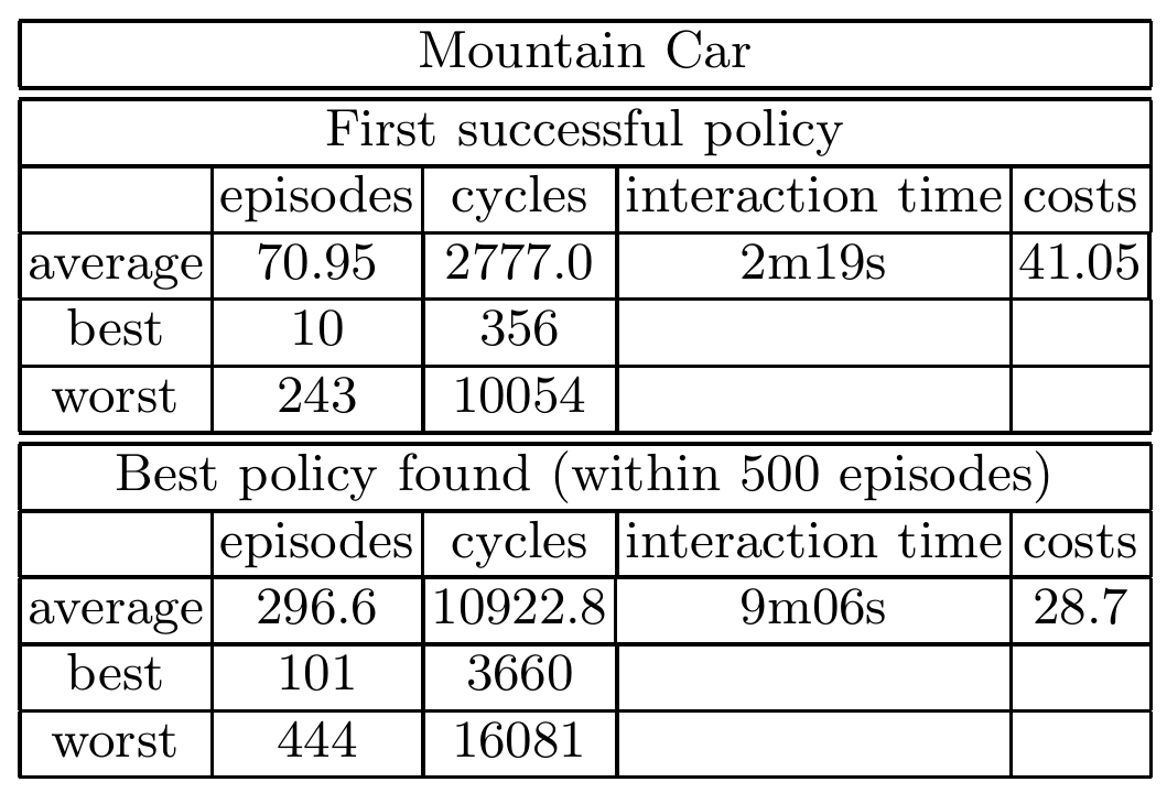
To test our NFQ algorithm, we run 20 experiments, with each experiment having different initial starting states for generating the sample set $D$ and different initial weights for the multilayer perceptron. For each experiment, we train an agent for 500 episodes. In all 20 experiments, the agent was able to find a successful policy - a policy that can reach the goal state from all of the 1000 starting states. On average, it took 139 seconds for the controller to find a successful policy.

5.3 The CartPole Regulator Benchmark

In CartPole, the agent’s task is to keep the pole in an upright position and the cart in the target position by moving the cart left or right. Because this is a regulator problem, the episode does not terminate even when the agent reaches an upright position. The goal of the agent is to be at the target position for as long as possible while staying away from the forbidden region.

State	Condition	Cost
$S^+$	$x \in [-0.05, 0.05]$ and $\theta \in [-0.05, 0.05]$	0
$S$	$x \in [-2.4, 2.4]$	0.01
$S^-$	$x \not\in [-2.4, 2.4]$	1

Two actions are available to the agent: left (-10N) and right (10N).

Learning System Setup

To generate the sample set $D$, the initial states are drawn randomly such that $x \in [-1, 1]$, $\theta \in [-0.3, 0.3]$, and $x’ = \theta’ = 0$. The actions are selected greedily using the current Q-value function until a forbidden state is reached or the maximum episode length of 100 is reached. We also use the hint-to-goal heuristic, generating 100 artificial goal-region transition after each training episode.

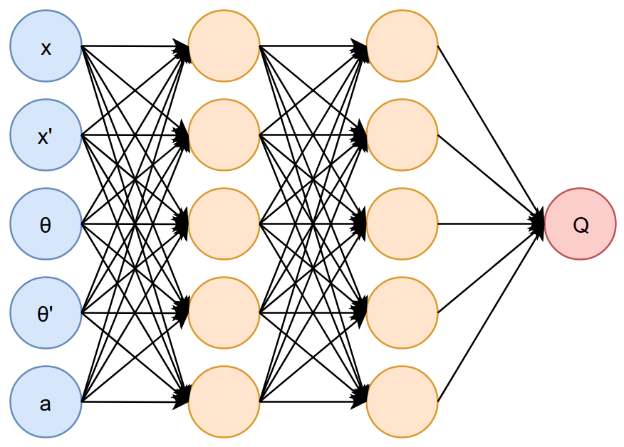
We use the same neural network architecture as the Pole Balancing problem and the Mountain Car problem, except the input layer has 5 nodes instead of 3 since the state is represented by 4 numbers $s = (x, x’, \theta, \theta’)$. The sigmoid activation function is used in all layers.

Results

The trained controller is tested on 1000 testing episodes, each with a maximum length of 3000 cycles. A controller is successful if at the end of the episode, the controller is in the goal region $S^+$.

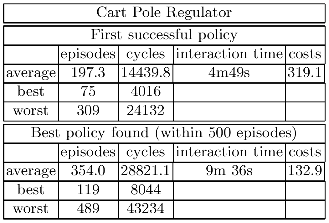
Let’s first look at the learning performance (the speed of learning). The experiments show that on average less than 5 minutes of interaction is needed to find a successful policy, while finding the optimal policy takes less than 10 minutes on average. To evaluate the control performance (the quality of the policy), we compare NFQ with a linear controller using a pole assignment method (classical control method). We see that the controller trained with NFQ has about $1/3$ the average cost of that of linear controller, showing that the NFQ controller reaches and stays in the goal region much better.

	Linear	NFQ
Average cost	402.1	132.9

6 Conclusion

This paper proposes NFQ, a memory based method to train Q-value functions represented by a neural network. We show that storing and reusing experiences allow for greater data efficiency and more reliable learning and convergence. NFQ was able to learn successfully on 3 optimal control problems using an identical neural network structure, showing that NFQ is at least somewhat robust against hyperparameters.

---

Final Thoughts

Questions

• In the Pole Balancing problem, there are 3 possible actions: left, right, or no-op. However, in the Mountain Car and CartPole problem, there are only 2 actions: left or right. What would happen if the no-op action was added?
• How viable is the hint-to-goal heuristic? It is very helpful in these three problems, but current deep reinforcement learning algorithms are tested on more complex environment suites such as Atari 2600. In such environments, the state representation is complex, and generating artificial data in the goal region can be difficult. Also, the state varies greatly within a state, so simply clamping the value in the goal region might not be as helpful.

Recommended Next Papers

• Playing Atari with Deep Reinforcement Learning (Mnih et al., 2013) [Arxiv]